A randomized algorithm

The closest pair problem

The closest pair of points problem is: given $n$ points, find the pair with the smallest Euclidean distance. Although it may seem trivial, it isn’t.

For example, given the following points, which pair is closest?

The correct answer is $(72, 34), (73, 39)$. The only way (at first) to check this is to try all pairs and compute the distances, keeping the smallest. That’s $O(n^2)$ operations. Can we do better?

In fact, yes. There is an algorithm that uses the divide and conquer technique, splitting the problem in half recursively and ultimately solving it in a total of $O(n \log n)$ operations, which is a significant improvement.

Can we improve it even further? We can, but only up to a point. There is a lower bound of $O(n \log \log n)$, so we can’t beat that.

So, is that the end of this blog post? Actually, that bound is for deterministic algorithms, so we can’t have an algorithm that is always faster and always works; but nothing stops us from having an algorithm with some probability of failure, or with some (arbitrarily small) probability of ending up as slow as $O(n \log \log n)$.

Linear time randomized algorithms

A randomized algorithm with linear expected time

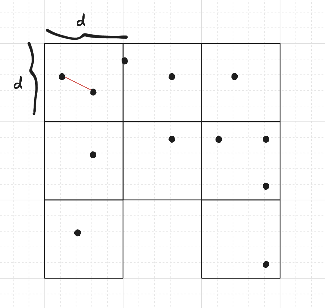
An alternative method, originally proposed by Rabin in 1976, arises from a very simple idea to heuristically improve the runtime: We can divide the plane into a grid of $d \times d$ squares, then it is only required to test distances between same-block or adjacent-block points (unless all squares are disconnected from each other, but we will avoid this by design), since any other pair has a larger distance than the two points in the same square.

We will consider only the squares containing at least one point. Denote by $n_1, n_2, \dots, n_k$ the number of points in each of the $k$ remaining squares. Assuming at least two points are in the same or in adjacent squares, and that there are no duplicated points, the time complexity is $\Theta\!\left(\sum\limits_{i=1}^k n_i^2\right)$. We can look for duplicated points in expected linear time using a hash table, and in the affirmative case, the answer is this pair.

Proof. For the $i$-th square containing $n_i$ points, the number of pairs inside is $\Theta(n_i^2)$. If the $i$-th square is adjacent to the $j$-th square, then we also perform $n_i n_j \le \max(n_i, n_j)^2 \le n_i^2 + n_j^2$ distance comparisons. Notice that each square has at most $8$ adjacent squares, so we can bound the sum of all comparisons by $\Theta(\sum_{i=1}^{k} n_i^2)$. $\square$

Now we need to decide on how to set $d$ so that it minimizes $\Theta\!\left(\sum\limits_{i=1}^k n_i^2\right)$.

Choosing d

We need $d$ to be an approximation of the minimum distance $d$. Richard Lipton proposed to sample $n$ distances randomly and choose $d$ to be the smallest of these distances as an approximation for $d$. We now prove that the expected running time of the algorithm is linear.

Proof. Imagine the disposition of points in squares with a particular choice of $d$, say $x$. Consider $d$ a random variable, resulting from our sampling of distances. Let’s define $C(x) := \sum_{i=1}^{k(x)} n_i(x)^2$ as the cost estimation for a particular disposition when we choose $d=x$. Now, let’s define $\lambda(x)$ such that $C(x) = \lambda(x) \, n$. What is the probability that such choice $x$ survives the sampling of $n$ independent distances? If a single pair among the sampled ones has distance smaller than $x$, this arrangement will be replaced by the smaller $d$. Inside a square, about $1/16$ of the pairs would raise a smaller distance (imagine four subsquares in every square; using the pigeonhole principle, at least one subsquare has $n_i/4$ points), so we have about $\sum_{i=1}^{k} {n_i/4 \choose 2} \approx \sum_{i=1}^{k} \frac{1}{16} {n_i \choose 2}$ pairs which yield a smaller final $d$. This is, approximately, $\frac{1}{32} \sum_{i=1}^{k} n_i^2 = \frac{1}{32} \lambda(x) n$. On the other hand, there are about $\frac{1}{2} n^2$ pairs that can be sampled. We have that the probability of sampling a pair with distance smaller than $x$ is at least (approximately)

so the probability of at least one such pair being chosen during the $n$ rounds (and therefore finding a smaller $d$) is

(we have used that $(1 + x)^n \le e^{xn}$ for any real number $x$, check Bernoulli inequalities).
Notice this goes to $1$ exponentially as $\lambda(x)$ increases. This hints that $\lambda$ will be small for a poorly chosen $d$.

We have shown that $\Pr(d \le x) \ge 1 - e^{-\lambda(x)/16}$, or equivalently, $\Pr(d \ge x) \le e^{-\lambda(x)/16}$. We need to know $\Pr(\lambda(d) \ge \text{something})$ to be able to estimate its expected value. We notice that $\lambda(d) \ge \lambda(x) \iff d \ge x$. This is because making the squares smaller only reduces the number of points in each square (splits the points into other squares), and this keeps reducing the sum of squares. Therefore,

(we have used that $E[X] = \int_0^{+\infty} \Pr(X \ge x) \, \mathrm{d}x$, check Stackexchange proof).

Finally, $\mathbb{E}[C(d)] = \mathbb{E}[\lambda(d) \, n] \le 16n$, and the expected running time is $O(n)$, with a reasonable constant factor. $\square$

Implementation of the algorithm

The advantage of this algorithm is that it is straightforward to implement, but still has good performance in practise. We first sample $n$ distances and set $d$ as the minimum of the distances. Then we insert points into the “blocks” by using a hash table from 2D coordinates to a vector of points. Finally, just compute distances between same-block pairs and adjacent-block pairs. Hash table operations have $O(1)$ expected time cost, and therefore our algorithm retains the $O(n)$ expected time cost with an increased constant.

Check out this submission to Library Checker.

#include <bits/stdc++.h>
using namespace std;


using ll = long long;
using ld = long double;


struct pt {
	ll x, y;
	pt() {}
	pt(ll x_, ll y_) : x(x_), y(y_) {}
	void read() {
		cin >> x >> y;
	}
};

bool operator==(const pt& a, const pt& b) {
    return a.x == b.x and a.y == b.y;
}


struct CustomHashPoint {
	size_t operator()(const pt& p) const {
		static const uint64_t C = chrono::steady_clock::now().time_since_epoch().count();
		return C ^ ((p.x << 32) ^ p.y);
	}
};


ll dist2(pt a, pt b) {
	ll dx = a.x - b.x;
	ll dy = a.y - b.y;
	return dx*dx + dy*dy;
}


pair<int,int> closest_pair_of_points(vector<pt> P) {
    int n = int(P.size());
    assert(n >= 2);

    // if there is a duplicated point, we have the solution
    unordered_map<pt,int,CustomHashPoint> previous;
    for (int i = 0; i < int(P.size()); ++i) {
        auto it = previous.find(P[i]);
        if (it != previous.end()) {
            return {it->second, i};
        }
        previous[P[i]] = i;
    }

	unordered_map<pt,vector<int>,CustomHashPoint> grid;
	grid.reserve(n);

	mt19937 rd(chrono::system_clock::now().time_since_epoch().count());
	uniform_int_distribution<int> dis(0, n-1);

	ll d2 = dist2(P[0], P[1]);
	pair<int,int> closest = {0, 1};

	auto candidate_closest = [&](int i, int j) -> void {
		ll ab2 = dist2(P[i], P[j]);
		if (ab2 < d2) {
			d2 = ab2;
			closest = {i, j};
		}
	};

	for (int i = 0; i < n; ++i) {
		int j = dis(rd);
		int k = dis(rd);
		while (j == k) k = dis(rd);
		candidate_closest(j, k);
	}

	ll d = ll( sqrt(ld(d2)) + 1 );

	for (int i = 0; i < n; ++i) {
		grid[{P[i].x/d, P[i].y/d}].push_back(i);
	}

	// same block
	for (const auto& it : grid) {
		int k = int(it.second.size());
		for (int i = 0; i < k; ++i) {
			for (int j = i+1; j < k; ++j) {
				candidate_closest(it.second[i], it.second[j]);
			}
		}
	}
 
	// adjacent blocks
	for (const auto& it : grid) {
		auto coord = it.first;
		for (int dx = 0; dx <= 1; ++dx) {
			for (int dy = -1; dy <= 1; ++dy) {
				if (dx == 0 and dy == 0) continue;
				pt neighbour = pt(
					coord.x  + dx, 
					coord.y + dy
                );
				for (int i : it.second) {
					if (not grid.count(neighbour)) continue;
					for (int j : grid.at(neighbour)) {
						candidate_closest(i, j);
					}
				}
			}
		}
	}

	return closest;
}

An alternative randomized linear expected time algorithm

Now we introduce a different randomized algorithm which is less practical but very easy to show that it runs in expected linear time.

• Permute the $n$ points randomly
• Take $\delta := \operatorname{dist}(p_1, p_2)$
• Partition the plane in squares of side $\delta/2$
• For $i = 1,2,\dots,n$:
  • Take the square corresponding to $p_i$
  • Iterate over the $25$ squares within two steps to our square in the grid of squares partitioning the plane
  • If some $p_j$ in those squares has $\operatorname{dist}(p_j, p_i) < \delta$, then
    • Recompute the partition and squares with $\delta := \operatorname{dist}(p_j, p_i)$
    • Store points $p_1, \dots, p_i$ in the corresponding squares
  • else, store $p_i$ in the corresponding square
• output $\delta$

The correctness follows from the fact that at any moment we already have some pair with distance $\delta$, so we try to find only new pairs with distance smaller than $\delta$. Since each square has side $\delta/2$, a candidate pair can be at most at a distance of $2$ squares, so for a given point we check candidates in the surrounding $25$ squares. Any point in a square further away will always give a distace larger than $\delta$.

While this algorithm may look slow, because of recomputing everything multiple times, we can show the total expected cost is linear.

Proof. Let $X_i$ the random variable that is $1$ when point $p_i$ causes a change of $\delta$ and a recomputation of the data structures, and $0$ if not. It is easy to show that the cost is $O(n + \sum_{i=1}^{n} i X_i)$, since on the $i$-th step we are considering only the first $i$ points. However, turns out that $\Pr(X_i = 1) \le \frac{2}{i}$. This is because on the $i$-th step, $\delta$ is the distance of the closest pair in $\{p_1,\dots,p_i\}$, and $\Pr(X_i = 1)$ is the probability of $p_i$ belonging to the closest pair, which only happens in $2(i-1)$ pairs out of the $i(i-1)$ possible pairs (assuming all distances are different), so the probability is at most $\frac{2(i-1)}{i(i-1)} = \frac{2}{i}$, since we previously shuffled the points uniformly.

We can therefore see that the expected cost is